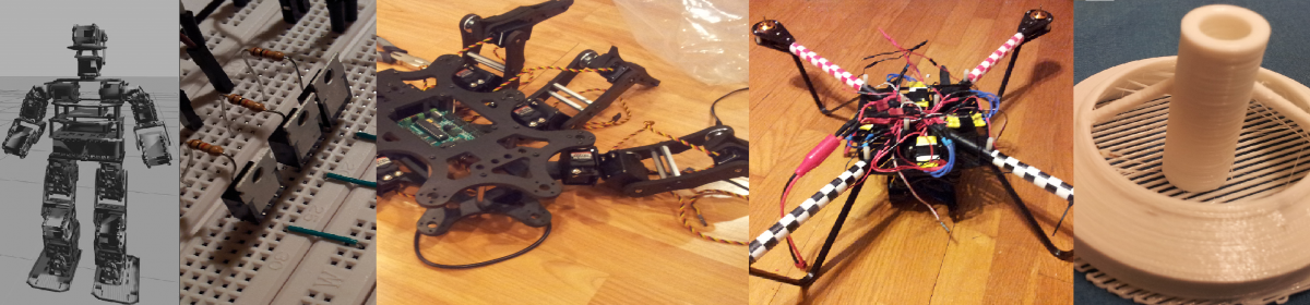
Overview

As part of the course ‘SYDE 652 – Multibody Dynamics’, a classmate and I attempted to identify the inertial parameters (mass, inertia, and offset of center-of-mass) of a robot arm. We were able to calculate several parameters, which lead to estimating torque requirements with less error than using provided parameters (compared against joint sensor readings).

My work in this project involved the mathematics/implementation of identifying the parameters as a least-squares problem, design of experiment, and analysis of convergence and error.

This project served as an excellent introduction not only to this area of rigid-body dynamics, but also to the Pinocchio programming library, automatic differentiation, and design-of-experiment.

Description

Creating a Least-Squares Problem

From the 2016 Spring Handbook of Robotics by Siciliano and Khatib, the relationship between the forces acting on each joint of the robot, and the inertial parameters of masses beyond said joint, is linear. This linear equation can be stacked for each joint, and again for multiple poses and actions, to create a linear system which can be solved for the parameters (phi):

$\tau = A*\Phi$

To create the elements of this equation, I used the Pinocchio rigid body dynamics library. This library can perform the inverse dynamics calculation required to calculate expected joint torques give current joint position, speed, and a guess of inertial parameters.

I then made use of Pinocchio’s templating feature and used CppAD as an Algorithmic Differentiation tool. The algorithmic differentiation allowed me to take the jacobian of rigid body dynamics calculations in terms of the inertial parameters, extracting the A matrix.

Design of Experiment

Experimentally determining the inertial parameters of a system is a problem that requires many samples gathered during relatively ‘expensive’ motions performed on the robot.

To deal with this, I tested several poses of the robot in simulation. At each of these simulated poses, I could calculate the new addition to the stacked regressor matrix. This regressor matrix can be used to calculate the variance of the inertial parameters upon solving the linear equation:

$\Sigma= noise^2 (A^T)^{-1}$

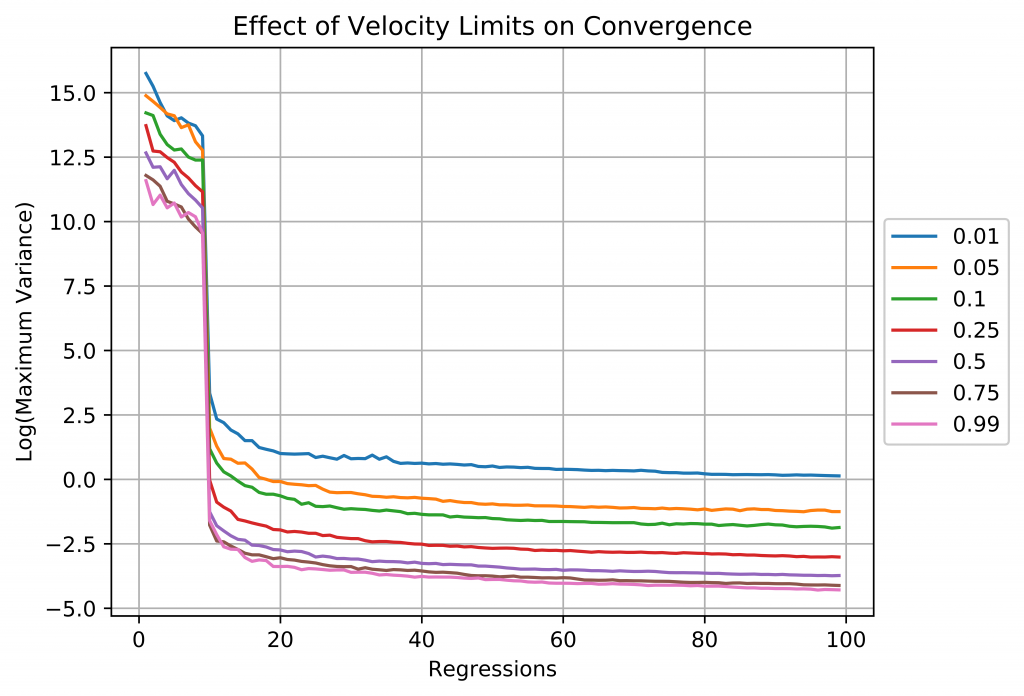
Choosing the configuration which leads to the smallest value for the largest variance, or the condition number of A, leads to faster convergence of the solution.

The figure below shows how the variances converge after a given number of samples (‘regressions’) and maximum commanded joint velocities as a percentage of maximum physical joint velocities. The graph shows that higher speeds lead to greater convergence, which can intuitively be explained by exciting dynamic parameters to a greater extent.

Results and Error Analysis

We were able to solve for a small subset of the robot parameters. Using these new parameters, we were able to calculate the expected joint torques at several poses with less error than our initial (provided by the manufacturer) parameters. To end the project, I performed further error analysis and identified ways to improve the process.

The first improvement which can be made would be to recast the problem as solving for deviations to our provided parameters instead of solving for the parameters themselves. This would have the effect of constraining the problem, as many parameters exist only as linear combinations of each other, and cannot be mathematically distinguished otherwise. In fact, while our method lead to less error in calculating torques, some estimated parameters were wildly off their provided values. This recasting would have a normalizing effect.

$\begin{bmatrix}\Delta \tau \\ 0 \end{bmatrix} = \begin{bmatrix} A \\ I \end{bmatrix} \Delta \Phi$

I also looked into many other sources of error, with none explaining the major difference in the parameters we calculated.

Sensor error effects
Sensor delay effects
Effects of exploring more states in simulation